
Price Optimisation through Machine Learning for Retail Stores
Introduction
Price optimisation refers to determining the prices of products/services such that the company can achieve its business objectives. In recent times, there have been major technical advancements in this field with more reliable and faster techniques. This has led to strong competition among the market players in having an edge over others in terms of their pricing strategies so as to attract most customers along side having considerable profits. The table below lists down some of the probable models which can be used for Price Optimization.
| Model | When to Use |
| Qualitative Approach | When the product is new and no past data is available. |
| Causal Model | When some cause-effect relationship exists between independent and dependent variables. |
| Time Series Model | When past data with some seasonality or pattern is available. |
One robust solution for optimal pricing is provided by Machine Learning. This involves the use of past customer and market data in building a model to predict the future demand of the products and later on the most optimal price for them. The model is used to find the best product price points in real time.
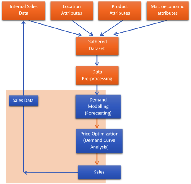
For a retail store, the factors considered while pricing their products are the demographics of that region, past sales data, and the market trends. The sales (by volume) data at the product level for the past one year is collected and gathered in a single data set. We then handle the issues of missing data, inconsistent data or irrelevant data in the dataset. We also structure the data such that all the final pre-processed values are in the form that can be processed by our model being built. An analysis of the data is also done to check the distribution of demand across the past year. In our case we obtain that product specific demand doesn’t show any linearity but are simple curves.
We now build a Causal model on this past data following the approach of Regression to forecast the demand of the individual products. A Causal forecasting technique is one which assumes a cause-effect relationship between the variable to be forecast and the various independent variables. Also, we choose Causal forecasting over Time Series forecasting because the former allows granular forecasting at the product level with higher accuracy as compared to the Time Series technique. The Causal model considers all the possible factors which can impact the dependent variable which would be otherwise difficult for a normal human to consider all at once. In our case, we take the internal sales data as well as external data points like market surveys, product features, and macroeconomic indicators.
The Regression approach estimates a function between the independent and dependent variable using the least squares method to define the interactions between them. We here use the Polynomial Regression model as the sales data of the past year in our data does not show linearity in its distribution.
We split the data into 80% as training data and the remaining as the test data. The model is then fit to the data and after training on that data the polynomial regression function is established which provides the relationship between the sales data of each product and their corresponding influencing factors. Further, the predictions are performed for the test data and the prediction thus obtained is evaluated on the basis of RMSE and R2 -score to understand the accuracy.
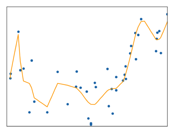
Source: https://towardsdatascience.com/polynomial-regression-bbe8b9d97491
Once the model is trained and tested, we finally perform the forecast at product level for future dates. The forecasted demand/sales value is later used to find the optimal price of the products based on the objective of the business. The most common idea to perform optimal price predictions is to evaluate on which price points can give the business the most margin or we can say the profit. For this purpose, the concept of Demand curve is used here.

Source: https://www.tutor2u.net/economics/reference/revenues
A Demand curve is a graph plot between the Price of a good/service and the Quantity demanded for a period of time for that product. This curve forecasts the revenue at every price point which is area under the curve at that point. The formula used is:
Revenue = Price per unit * Quantity demanded
Benefits of Price Optimisation
The predicted demand is plotted on the demand curve to find the price point with which the store can achieve its revenue targets (or, the margin targets) for each product. This optimisation of price can be done at regular periods or in real time as per the choice and the requirements of the store owners.
The opportunity to focus on various goals such as the sales margin and other such conversions make financial benefits clearly visible for business and add up to its growth and expansion. Price optimisation also helps the retail business adapt to market trend changes with automatic and quick price adjustments. Optimized product prices make the business abled to take efficient and quick decisions on discount offers or marketing and promotion investments.
Last but not the least, this automatic pricing model reduces manual efforts and removes the risk of human errors, thus, the system can be relied upon by the retail executives. Moreover, a further development can be that we can study the response of the consumers towards the price shifts of the products and use that analysis result also for pricing decisions.
Follow