
Time Series 101 : Everything you need to know about Time Series
Time is always an important factor when it comes to observing patterns or forecasting trends, be it predicting stock prices or future sales of products. For example, if the expected sales of a product are supposed to take a hit, a company can take various measures to stunt that fall or even improve the performances. As the name clearly indicates, time series is used to analyze data over a period of time. A time series, in theory, is a series of data points ordered in time. In this framework, time is usually the independent variable and the end product is a forecast of data for the future.
To begin with, historical sales data is used to create a time series model, which will help forecast data for the forthcoming year.
But before fitting the data to the model, the data needs to be made stationary, if it’s not. Different transformations are done to achieve the same. Data normalization is one such method. There are various tests like the Dickey-Fuller test to check if the data is stationary or not. In this test, a hypothesis test is conducted to deduce if the data is stationary or not. Lastly, before we start creating the model, data will be pre-processed or in other words structured and cleaned, so that it can fit into the model seamlessly.
There are various modeling techniques with which a time series model is created. The Seasonal autoregressive integrated moving average model is one such technique which can take care of a lot of complexities in data, including it being non-stationary or seasonal.
Seasonal autoregressive integrated moving average model (SARIMA) is actually a combination of different models.
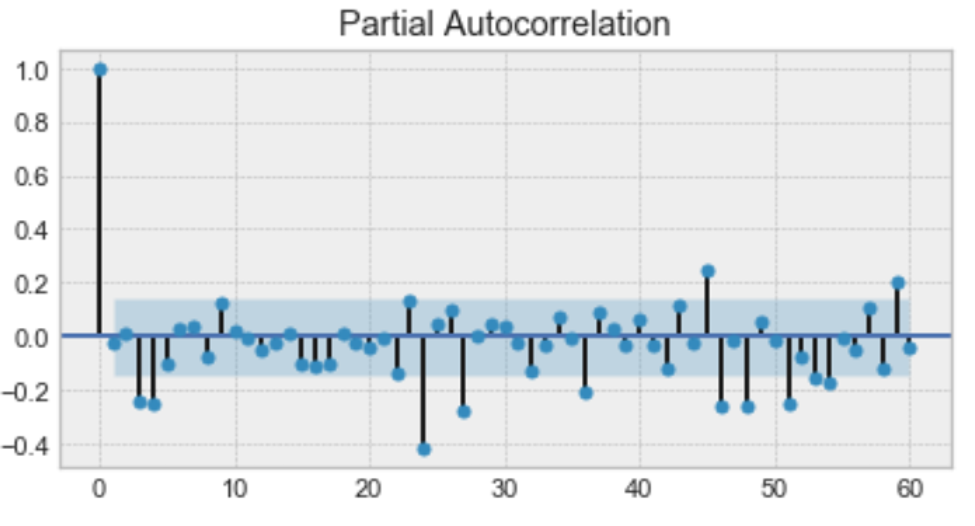
The autoregression model (p) is put to use first, where p determines the longest time lag post which data has little to no correlation. This value is found using the partial autocorrelation plot. The partial autocorrelation plot is a plot of the partial autocorrelation co-efficients between the series and time lags of itself.
Here, p should be 4.
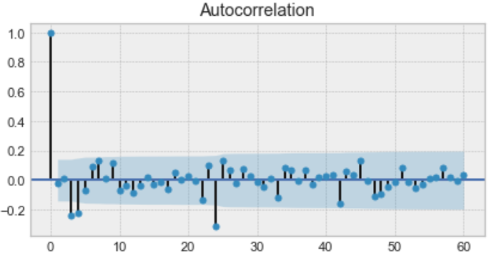
This is followed by using the moving average model (q), which determines the biggest time lag after which other lags are not significant. This is found by referring to the autocorrelation plot.
Just like in the partial autocorrelation plot, q should be 4 here.
The order of integration (d), the magnitude of which indicates if the series is stationary or not, is the last model implemented. Together, combining all these models gives us the SARIMA model.
Follow